Complete Implementation and Intuition Behind Linear Regression from scratch using python

Linear Regression is a simple and most popular Machine Learning Algorithm that comes very first when you are beginning with your data science journey. It basically identifies the relationship of independent variables with dependent variables. In this tutorial, we are going to understand the complete mathematical working of the linear regression algorithm and how it predicts the relationship. we will build an algorithm manually and predict the result as well we will see the code with an inbuilt Python library and how it makes easy development.

Table Of Contents

1. Brief Overview of Linear Regression Algorithm
2. How does linear regression work?
3. Implement linear regression from scratch using plain python
4. Linear regression algorithm using in-built classes
5. End Notes

Overview about linear regression algorithm

Since Linear Regression depicts the linear relationship, means it shows how the dependent variable is changing(increase or decrease) concerning independent variables. so, the linear regression plots a straight line that plots the best possible points and finds the relationship such that the distance between the plotted line and point is minimum.

👉 Before diving into calculations, the first brief about the equation of straight line because the working of linear regression depends on this only. so the equation of straight line suggests that 

     Y = Mx + C.

        here,  M is a slope of a line 

                   C is any constant or Y Intercept.

The same equation is followed by Linear regression where Y is the dependent variable and X is the Independent variable. M and C are the coefficients and intercept of the line. You will find the same equation written in different ways in different articles.

     Y = ax + b

OR

     Y =  b0 + b1 x1

so, all these equations are the same, do not get confused between these equations.

Maths and Intuition behind linear regression with example

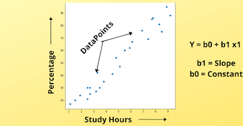
To understand the above equation and the mathematical intuition behind the linear regression algorithm let's take a simple example. Here is a simple case study of students with their study hours concerning percentage scores. we want to find that if a student studies at any number of hours a day then, how many minima or maximum percentage he will able to secure. 

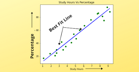
we have plotted various points on a graph stating student percentage scores concerning study hours. Now, we have to identify the relationship between these points, so what Linear Regression does is to Plot a Best Fit Line. The main aim of Linear Regression is to find the Best Fit Line that passes through all the data points such that the distance between the line and data points is minimum.

This distance is known as an error which we will calculate and it will be known as False prediction(mistake) of algorithm and we want to minimize this error to make an accurate prediction.

This Blue line is known as Best Fit Line, shown in the above image and we have to find this line only. In short, if it seems confusing only understand that, we have to draw a line that will best fit all these data points in such a way that, the error between these points and line is minimized.

The main thing to keep in mind while drawing the best fit line is Overfitting means do not accurately fit the line to all training data otherwise the model will overfit to training data and perform worse on new data(test data).

The equation written above is used to fit the straight line to a graph. people who have studied straight line chapters in mathematics will be familiar with the equation. b0 is a constant, which is fixed and b1 is a score of a plot, or it's merely a coefficient.

👉 So, let's see what b0 is in a graph, suppose that all the students are capable to cross or bring at least a 20 percent score, so we can set it as a base score and the best fit line will start from here.

👉 So, now take a random study hour, consider we want to find the minimum percentage that can be secured if Shyam studies 3.5 hours a day. so we can easily plot 3.5 study hours and can see the corresponding Y-axis value as a minimum percentage that can be secured if he studies 3.5 hours a day.

Calculations in linear regression

Now, we have understood the working of Linear Regression. let's just see how does it calculates the coefficient and then we will implement it in Python.

    Y = b0 + b1 x  

    b1 = sum((x(i) - mean(x)) * (y(i) - mean(y))) /  sum(( x(i)  -  mean(x)) ^2 )  

    OR

    

    b1 = covariance(x,y) / variance(x)       #Slope    

    b0 = mean(y) - b1 * mean(x)                 # Intercept

Now, you know how to find the covariance of independent variables, find the mean of variable and under summation subtract the mean of a variable from each observation with respect to a dependent variable. we also refer to mean as a bar and the formula we see written as:

    covar = sum((x - x_bar) * (y - y_bar))  

This bar is the mean (average) of whole observations. And finding the variance is simple and it can also be written as:

    var = sum((x - x_bar)^2)

Build Linear Regression Algorithm manually using Python

Now, we will implement the complete linear regression algorithm and understand it's working with code to know how it calculates the coefficients and intercepts and builds the best fit line for us.

from math import sqrt

#calculates mean value of a list of numbers

def mean(values):

    return sum(values) / float(len(values)) 

                                                                                                                                                

#Calculate Covariance between X and Y

def covariance(x, mean_x, y, mean_y):

    covar = 0.0

    for i in range(len(x)):

        covar += (x[i] - mean_x) * (y[i] - mean_y)

    return covar

                                                                                

#Calculate the Variance of a list of numbers 

def variance(values, mean):

    return sum([(x - mean) ** 2 for x in values])    # (x- x_bar)^2

                                                                                             

#Calculate Coefficients as b0 & b1

def coefficients(dataset):

    x = [row[0] for row in dataset]  #Independent

    y = [row[1] for row in dataset]  #Dependent

    x_mean, y_mean = mean(x), mean(y)

    # Calculate Slope

    b1 = covariance(x, x_mean, y, y_mean) / variance(x, x_mean)

    #Calculate Intercept / coefficient

    b0 = y_mean - b1 * x_mean

    return [b0, b1]

                                                                                                                                                             

# Simple Linear Regression Algorithm

def simple_linear_regression(train, test):

    predictions = []

    b0, b1 = coefficients(train)   #find the coeffiecents

    #print(b0, b1)

    for row in test:

        yhat = b0 + b1 * row[0]

        print(yhat, row[0])              # predicted and actual output

        predictions.append(yhat)    #save the predicted value in list for error caclculation

    return predictions

                                                                                                                                                              

# to evaluate the result we required metric, so, let's build one simple metrics for evaluation

# calculate root mean squared error(RMSE)

def rmse_metric(actual, predicted):

    sum_error = 0.0

    for i in range(len(actual)):

        prediction_error = (actual[i] - predicted[i])

        sum_error += prediction_error ** 2

    mean_error = sum_error / len(actual)

    return sqrt(mean_error)

                                                                                                  

# evaluation the regression algorithm on training data

def evaluate_algorithm(dataset, algorithm):

    test_set = []

    for row in dataset:

        row_copy = list(row)

        row_copy[-1] = None

        test_set.append(row_copy)

    predicted = algorithm(dataset, test_set)

    print(predicted)

    actual = [row[-1] for row in dataset]

    rmse = rmse_metric(actual, predicted)

    return rmse

                                                                                                

#Test the simple Linear Regression 

dataset = [[1,1], [2,3], [3,4], [4,3], [3,2], [5,5]]  #when x=1, y=1 and so...

rmse = evaluate_algorithm(dataset, simple_linear_regression)

print("Root mean squared error, RMSE : %3f" %(rmse))

                                                                                                

Code Explanation:

Now, let's understand how our model will predict the performance by understanding the working of each and every function. So, we have taken a simple dataset and passed it to evaluate function along with the name of the algorithm. so, the first dataset will be split into 2 parts training and testing. For demonstration purposes only we are training it on a complete dataset and creating a copy of it for a test. But we are keeping the value of only x and y as None. so train and test become as:

    train = [[1,1], [2,3], [3,4], [4,3], [3,2], [5,5]]  

    test = [[1, None], [2, None], [3, None], [4, None], [3,None], [5,None]]  

👉 If you want to understand the concept of training and testing then refer to the Regression Analysis article. 

Now we will find the value of this y(None) in the test set to know how well our model(linear Regression) performs. After the split into train and test, both the dataset will go to the simple_linear_regression algorithm function. And first, it will calculate the coefficients as b0 and b1 with the help of the same formula as we have written. When it will get the coefficients it will calculate yhat which is our predicted variable as:

        yhat = b0 + b1 * row[0].

As you will run this you will get the output something like:

   [[1, 1.19], [2, 1.67], [3, 2.27], [4, 3.56], [3,3.21], [5,4.6]]

Now, we can see the output corresponding to each x. but we are getting the difference as corresponding to 1 it should calculate 1, but we got 1.19, so this difference(1.19-1) is known as an error which we are calculating with help of RMSE(root mean squared error) metrics

    rmse = sqrt( sum(y - (b0 + b1x)^2) / n )

Where, bo+b1x = predicted value

               y = actual value

               n = total input features    

We take the square of the error to avoid the cancellation of negative and positive values because we sum up all these errors to calculate the mean error of all the input features which we conclude as a complete error of the dataset.

👉 You do not have to take all this load and implement all functions again and again. To implement all this we have a library function in python known as LinearRegression which is present under the sciket-learn library.

Implement Linear Regression Algorithm using Library Function

You do not need to worry about all this code and do need to write again and again all this function. There is a great library in Python which has all the classes and functions regarding Machine Learning stuff. And It consists of a class as LinearRegression under linear_model package which you can directly import and use.

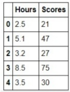
This is necessary for you to understand the background details of the algorithm, how actually it works, or what mathematics is working behind it. Now, we are having a dataset of student study hours corresponding to a percentage score that we have to predict.

Dataset:  You can download the dataset from here.

let's build our model using a simple linear regression algorithm.

#import libraries

import pandas as pd       #for reading and data manipulation

from sklearn.linear_model import LinearRegression

from sklearn.metrics import mean_squared_error

#Load the dataset

data = pd.read_csv('student_marks.csv')

#separate the independent and dependent variables

x = data.iloc[:, :-1]

y = data.iloc[:, 1]

#split into train and test set

x_train, x_test, y_train, y_test = train_test_split(x,y, test_size=0.2, random_state=0)

#train a model

lin_reg = LinearRegression()   # create an object of algorithm

lin_reg.fit(x_train, y_train)

#testing

y_pred = lin_reg.predict(x_test)

#check the performance of model

print("Model Performance", lin_reg.score(x_test, y_test))

Code Explanation

This is a simple code directly you have to import use in python. First, we load a dataset, split it into train and test sets as 80 percent of data will come in the train set and remaining 20 percent of data as the test set. we train the algorithm using the train set and function which is used to give train data to an algorithm that is fit(). Then, we predict outputs using predict() function and pass the testing data, and finally, we measure the model performance using the mean squared error metric.

Summary

👉 Linear Regression is a simple and most important algorithm which helps in the prediction of continuous values and depicts the relationship of independent variables and dependent variables. 

👉 Now, I hope that we are crystal clear with the working and implementation of simple linear regression and what mathematics work behind the complete algorithm. If you don't get it then please go through it again, it's so simple mathematics that you can easily solve. If you have any kind of queries, please post them in the comment section, I will be happy to solve your queries.
so, guys stay calm, keep learning, and keep exploring things.

Thank You!..