Hello and welcome to an amazing blog where we will build our first end-to-end machine learning project from developing to deploying completely from scratch. When I started my Machine learning journey then this was the first project that today I will represent in front of yours that how I deal with data and reached the end results. Before that time on Machine Hack data science Hackathon was going on and the problem statement was to predict the doctor consultation fees. By understanding the problem statement, I was excited to solve and apply whatever I have done so far. The excitement also came from seeing the leaderboard that the winner of the Hackathon has scored 76.16 percent accuracy. so, I have started working on it and tried to deploy it on Heroku using Flask. Check the deployed app here.
In this tutorial, We will solve the complete problem statement and build a different model to improve performance and I will be explaining my approach to deal with problem statements throughout this tutorial so let's get started.

Problem Description
We all visit a doctor in an emergency or in an uncomfortable situation and find the consultation fees that the doctor charge is too high. This is a major problem in metropolitan or tier-1 cities like Chennai, Bangalore, Mumbai, Calcutta, Delhi, etc. So as data scientists can record some data of these cities and build a generic model that could predict a doctor's consultation fees for us to assure that the fees he/she is charging are valid.
After understanding the problem description, let's jump into the approaching part of a project and understand the basic features of the data we are provided with.
Download the dataset from here.
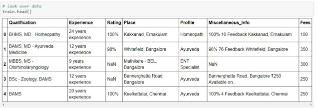
The dataset we have is small with 5961 rows and 7 unique columns(features).
- Qualification of doctor
- Experience of the doctor in years
- Profile of doctor
- Ratings that were given by patients
- Miscellaneous information that contains other information about a doctor
- Place(area and city of doctor clinic location)
- Fees Charged by the doctor(Dependent Variable)
Let's start implementing this in our Jupyter Notebook
1) Import all the libraries
we will be requiring NumPy and pandas for mathematical computation and data manipulation. And matplotlib with seaborn to visualize the data with interactive plots. Also, import the re module to deal with text data and ignore all the warnings.
2) Load Dataset
The dataset is in excel format so use the pandas read excel method to load the training and test dataset. after loading just see the shape and head of the dataset to have a near view of the data we have.

3) Exploratory Data Analysis(EDA)
There can be lots of analysis and preprocessing steps which can be assumed by observing the dataset because all the features we have are categorical except the target variable(Fees). let's start processing and analyzing the dataset with various steps such as univariate analysis, bivariate analysis, Imputing missing values so will place all such steps under EDA.
These steps can be divided into different ways and Preprocessing, Feature Engineering, which is done in different tasks. Let us check missing values in data first and move with univariate analysis.
There are missing values in the Rating and Miscellaneous information feature. A small amount of missing value is also present in the Place column.
Experience Column: Extract the exact numeric year of experience from the experience column which is categorical.
Place Column: replace the small number of missing values in the place column with "Unknown" and extract City and Locality as a different feature from the Place variable. And drop the place variable as now we do not require it anymore.
Rating Column: we will fill all the missing values with -1 percent and then, extract the Rating value from it without the percent sign.
After this, what I did is group the rating column into 10 groups as values less than 0 will be in the 0 groups while 0-9 percent will be in the 1 group, 10-19 percent values will be in the 2nd group, and so on. To divide the dataset into different bins we use the pandas cut() method.
use the cut() method when you want to segment the data values into bins. for example, a cut can convert age values to a group of the age range.
Qualification Column: There are lots of Qualification and doctors has done more than 1 qualification but most doctors have done one or two qualifications only. And we also have data of a doctor who has done 10 qualifications. as the data is too much messy about qualifications so we will take the top 10 qualifications which occur the most.
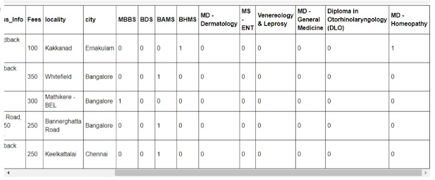
Here we extract the dictionary of each qualification with its count. Now we will extract the top 10 qualifications from this dictionary according to their frequency and after getting the top 10 qualifications, we will encode them in our data as a column and the doctor having any of the qualifications among these 10 there will be marked 1 else 0 in that column. A doctor having more than 1 qualification will be marked 1 in each column which qualification he has. After displaying the head of data you can see these features in your data.

City Column: first I remove the additional space from the name of cities. Then we have analyzed the number of places in a particular city we have. so we have the data of at least each place of that particular city, so by seeing the relation of place variable with target variable it is not so relevant. so we will not use the place column in our modeling and also it will create complexness in the deployment part.
4) Data Visualization
Now, let's do some bivariate analysis of data by visualizing it through plots which will provide us a better understanding of feature relationships and Hypotheses.
Before encoding a categorical variable let's have a look at their relationship with the target feature.

Now, let's look at the variation of fees with the city.

Look at the relation between doctor ratings concerning consultation fees. We always think that the doctor who has a high rating must be charging high fees. let's have a look.

- As Delhi, Bangalore, Mumbai, Chennai, Hyderabad are listed under tier-1 cities hence, the consultation fees are too high compared to other tier-2 cities.
- Doctor consultation fees are very high for a doctor who is having a profile as ENT Specialist and Dermatologist compared to Homeopathic or General Medicine.
- The Rating feature is very much an Interesting feature, as we have grouped it in 10 bins, the missing values are in 0 groups,s, and so on.
- As we can see the high rating does not relate to high fees(in fact low fees can be the reason for high ratings from the patients) and where the fees are charged so high have a rating between 30 to 60 percent. Here our assumption of hypothesis proved to be rejected.
5) Categorical Encoding
The qualification column is already converted to numeric and we have obtained the top 10 qualifications. now the city and profile column is only remaining to be encoded and the remaining Experience and Rating we have already converted to numeric.
After categorical encoding, just correct the names of some of the columns as they are having unnecessary spaces and hyphens in between.
Drop the Irrelevant features
The miscellaneous information column contains a lot of messy and missing data. And the data it contains is rating, place, and locality which is already with us so, we can drop this feature. We have already talked about the locality feature that does have a good correlation with the target variable so we will drop it out.
6) Prepare the Test Data before Modelling
Now, we have finished with preprocessing and feature engineering tasks. Let's clean the test data with the same methods as applied on train data and prepare it as it is train data to test the model's accuracy whatever we build.
I think you can apply all of this method on your own by seeing the above code to test data. If you are stuck anywhere then you can access to code at the link of the source code provided at end of this tutorial or you can also access the GitHub link from the footer of the web app deployed.
7) Model Building
Based on the hackathon site(Machine Hack), submissions are evaluated based on Root mean squared log error(RMSLE) and more especially on 1-RMSLE. I will use these metrics only for evaluating the model and we will create this using mean squared error metrics from the sciket-learn library.
- RMSLE:- The difference between the actual and predicted value and take the square summation of it and find the mean known as mean squared error. and only we take the log of predicted and actual values which is known as RMSLE.
Implement the RMSLE function
First import all the libraries then, we will make the RMSLE function. And for implementing the scoring function for cross-validation we use the make scorer method from sciket-learn.
Split dataset into train and test set
split the dataset on training and test set to check the model's performance.
Try different models on train and test and check the accuracy
Hyperparameter Tuning for Random Forest Algorithm
The hyperparameters for the KNN algorithm are less and after tuning, accuracy does not increase as of Random Forest so I have used Random Forest as the final algorithm for the project.
After hyperparameter tuning, check the performance and it is near about 79.3 which is not so good but from this particular Hackathon and winning accuracy point of view it is better so, we will save the model for further use in Flask development in the next tutorial.
8) Save the Model for Future use.
Download Source code
- Download the complete project source code from GitHub.
- You can also access the Kaggle Notebook of this complete project which you can copy and try different methods there themselves rather than on your local system.
- Check the web App and use it.
SUMMARY
The project was really very much interesting. I personally enjoyed it a lot during the preprocessing task and tried different plots and different techniques to impute it, you can also explore it in many ways as you want. This is an approach that I finalized for the particular project. This is part 1 of this project. In part 2 we will develop the flask web app to deploy this project on the cloud to be used by end-user.

