Beginners Guide to support vector machine (SVM) algorithm with python

Hello, and welcome to a wonderful blog on support vector machines. In this tutorial, we are going to understand the complete intuition behind the support vector machine and how it actually works along with implementation using python.

Table of Contents

1. Introduction to Support Vector Machine algorithm
2. Important terminologies related to the SVM algorithm
3. SVM with Non-Linear Data
4. Maths behind the working of support vector machine
5. Brief article summary

Introduction to Support Vector Machine (SVM Algorithm)

Support Vector Machine(SVM) is a supervised machine learning algorithm used for both regression and classification but mostly used for classification problems because It segregates the classes very nicely using a boundary called Hyperplane. we will understand it in detail.

let's understand some of the basic terminologies of support vector machines with an example.

Terminologies you need to know related SVM Algorithm

Suppose we have a binary classification problem, now what the SVM does is, basically creates the hyperplane and segregate the two classes with a parallel plane, as you can see in the image below.

1) Support Vectors

Support vectors are the points that are passing through the marginal plane. It is not one, that can be many. This helps us to determine the marginal hyperplane, if they are altered then, the hyperplane may get changed. So, they are the critical elements of a dataset.

2) Hyperplane

As in the above image for the classification problem you can see hyperplane as a line that linearly separates and classifies the data points. Intuitively, the far our data points lie to the hyperplane, the more confident we are that they have been correctly classified. Therefore we want the data points to be as far from the hyperplane as possible.

3) Marginal Axis. How do we choose the best Hyperplane?

Along with the hyperplane, it will draw two parallel planes passing through the nearest positive point and nearest negative point. Thus the main aim of SVM is to find the hyperplane with a maximum possible marginal axis that the distance between two parallel planes to hyperplane is more, which in place is very simple to classify the new data points.

This method works in binary classification problems of linear separate data points. we are using this technique to linearly separate the two classes.

SVM with non-linear data

Now, the question arises what if the data we have is non-linear? In order to solve this problem, the support vector machine uses the main technique known as SVM kernels. this kernel helps to convert the low dimensional data to high dimensional data. so that we will easily be classifying the two classes.

👉 for example, this is 2-d data and if we try to convert it into 3 dimensions then,  between that we will get a small hyperplane.

Please understand this basic concept guys, and remember that the main aim is to create the hyperplane with the maximum possible marginal axis because as margin will be greater, the more generalized our model is.

Maths Behind working of Support Vector Machine

Now, we have a basic understanding of support vector machines. So, let's understand the maths behind the working of the support vector machine. The first thing is to understand the basic difference between SVM and logistic regression.

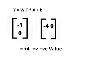
One thing to get in SVM is greater marginal distance. Let us consider a simple example of the above-given figure and consider the slope as -1. The equation of hyperplane is given by

                                        w.T * x + b = 0

    here, T represents the transpose of W. and slope(m) = -1.

we do transpose because we have to perform matrix multiplication. whenever we apply this equation in a downward direction, it's always going to be positive.

Whenever we compute this, it's always going to be positive. so, this is one scenario. And similar if we compute this in the top direction, it's always negative. and b is 0 in this case.

👉 Now, to compute the marginal distance, we can write the equation of both the part like this,

    W.T * X1 + b = -1 (negative side)

    W.T * X2 + b = 1 (positive side)

If we solve both the equation, the bias term will get cancel out, and the equation you will get as

    W.T(X2 - X1) = 2

Now, I have to remove this W of T, so we can remove it using the norm of W of T. remember that you cannot directly remove this, so we use norm. Now, we will write the equation as 

     W.T  (X2 - X1)   =  2 

      |W|                        |W|

This is our equation or optimization function, that needs to maximize.

(W, B) max  2        Optimizaton Function

                     |W|

One thing we know that whether it calculates a positive or negative value, it will consider or take it as +1 or -1 only.

such that,

   

    y[i] = 1      when   W.X + b   >=  1

    y[i] = -1    when    W.X + b  <=  -1

So,   y[i]  =  W.T  * X[i] + b[i]   > 1

We will get this final equation at last because -ve multiplied by -ve is positive and positive to positive is there. Now, if we compute our points with the above two-equation, it should be greater than 1. It is not greater than 1, Then it is a misclassification.

But, we have to not overfit the data in this particular way, because in the real-world problem statement, I will not be finding all this and the data would not be linear, there will be lots of overlapping. So the final output of this particular equation is, we take the min.

The max equation will be represented in form of min. Now we are wondering why we are taking min because we have to minimize the distance through derivatives to overcome overfitting.

we represent the equation as, 

(W*, b*) = min ||W|| + C

Σ E[i]

                                2

Here, we have added 2 parameters as C which is known as how many errors we have. And E[i] represents the value of error.

We can consider some 4 to 5 errors in the model because we have to create a generalized model. Thus this C parameter tells that how many errors can we consider in the model. Therefore, we are having a c number of errors so, we have to not change our hyperplane. and the parameter c is known as the regularization parameter. 

Changing a single point can directly affect the hyperplane and can alternate it, thus we follow this case.

Summary

This is complete intuition behind the working of SVM and how the maths behind this is derived. There will be many scenarios where some points will not fit, then you have to use the SVM kernel trick. In this tutorial, we have seen a complete understanding of the linear problem how to solve this using SVM. in the next article we will be exploring the intuition behind the kernel SVM.

keep learning, keep exploring and keep reading blogs.

Thank you!..